Problem
Class assignment four has us exploring the distribution fits laid out in chapter four and seeing how they fit real world data sets. We again use our speech signal and google stock as a basis for our analyses. From chapter four we are introduced to a number of distributions:
| Bernoulli | Binomial | Geometric |
|---|---|---|
| Exponential | Normal (Gaussian) | Uniform |
These different distribution models help us model random variables in things like our speech signal or google stock. What we hope to accomplish in this write up is to see how we can use these distribution models to predict an expected outcome.
Approach and Results
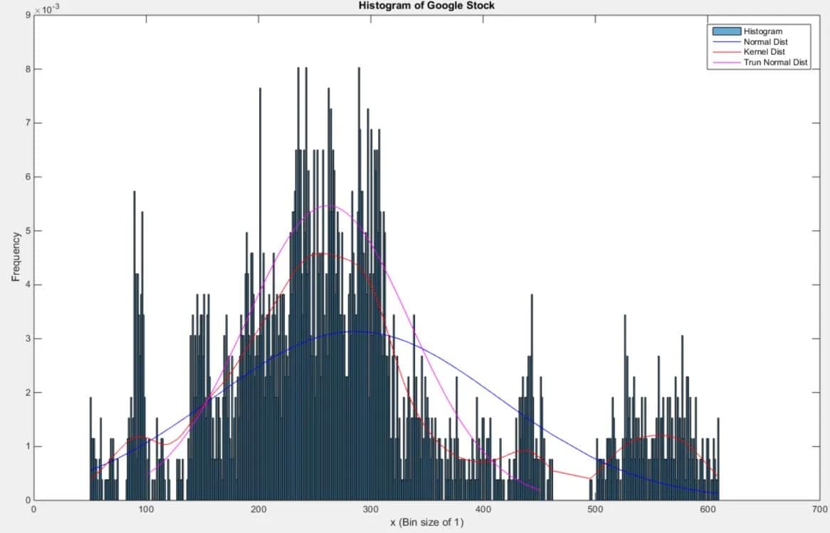
To begin the assignment we take our speech signal and find its histogram. Once we have a histogram (or pdf) of our speech signal, a good first approach to try a normal distribution. We lay our distribution on top of our histogram to see the fit.
Due to the possible ranges of our audio signal [-32768:32768] there are
many samples whose values become outliers when compared to the
mean/variance. Therefore, one may think the correlation between to be low.
Yet, our assumption of trying a normal distribution first pays off. With
the way our audio signal is constructed we see how most of our signal is
centered around zero. A normal distribution is also centered around the
mean making the correlation between the two high. In our analysis we
compared the histogram to normal distribution fit to find a mean squared
error between the two.