Problem
The purpose of this analysis is to take to see how variance changes if you were reading in real-time data. The analysis simulates for instance live tv broadcasts where the output signal is not completely known. Since we do not have all the data upfront, the variance of the signal will change as more of the signal comes in.
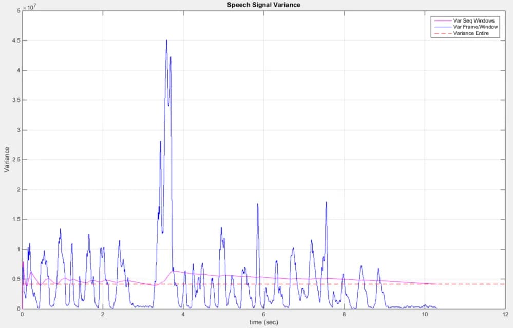
We will calculate our variance using three different approaches. For all analyses we will use both the speech signal and the Google Stock price. The first variance we calculate is the variance given the entire signal. We can find the variance by taking the second moments and subtracting the mean of the signal. This variance will be plotted as a horizontal line in our plots.
The second approach we take is simulating a streaming in data signal (such as our live TV broadcast). We begin by taking the first 10 samples and sequentially compute the variance one sample at a time. Therefore our samples start at 10 then 11, 12, 13, and so on. We plot this variance on the plot as our variance for the entire signal as a whole. The third approach will use a frame and window method which we have explored in previous assignments. We find the variance for a window of size 30 days at a time. Our frame shifts by a day at a time. We again plot the variance using this method on the same plane to perform comparisons with the previous variances we found. Overall, this assignment asks us to see how a mean/variance changes overtime.
Approach and Results
The different methods we proposed are all done for both our Google Stock price and the speech signal. The different methods highlight how the variance and mean change as time progresses for a live signal broadcast. The variance at the beginning of a signal may be largely different compared to the true actual variance.
First we see the variance if given the entire signal up front (red dotted line). The variance is rather high indicating that the Google Stock price ranges widely from the expected value (the mean). It is to be expected that we see a high variance since google stock price does not same at the price for an extending period of time. It is always changing.
If we pretend that our Google stock is being read in real time (one day at a time) we see that variance gradually increases (magenta line). As we expand our sample space both the mean and variance changes. For example, for the first ~100 days our variance is rather low since our variance and mean both increase. At around day 400 Google’s stock increases rather quickly which corresponds to stark increase in variance. As we incorporate more data into our sample space our values start varying more from the mean. We also should note where the magenta line is pretty steady. This no change in variance portion of the plot indicates that Google’s stock price did not change much during this time. Referencing Figure 1 for this range (day 1500 -> 2000) we observed that indeed Google’s stock is steady in price. Once we have the entire signal in our sample space [N = length (speech_signal)] we see our variance reach the true variance of the signal.