Introduction
In this experiment we will be introduced to open loop motor control. The point of this experiment is to use the tools at our disposal, i.e. MatLab and Simulink, to obtain the transfer function of the motors velocity using the data obtained experimentally. This lab also serves as an introduction to the extremely useful system identification toolbox.
Procedure
To begin we first build a DC motor step response model into Simulink. The input is a step and our output is the position and speed read in by the encoder.
After we pass our step input into the model we can start reading in data from the sensor. Since the DC motor takes in to inputs we have a gain block that gives us a predetermined speed. For an analysis we export our position data to our workspace. Outputting to the workspace will allow us to plot our position with respect to time. We also take the derivative of our position data so that we have the speed of the motor inside our workspace. The setup of the hardware is the same as previous experiment.
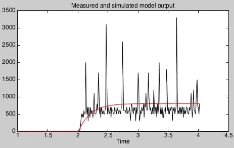
For the experiment we range our step response from 50, 150 to 255. To analyze
the data we plot our speed and position with respect to each one of our inputs.
From these plots we can find a first order transfer function. The transfer
function can be found by hand using an estimate of the DC gain (or steady state
value 𝐻(0)), and the time constant (𝜏). From these two values we can find
the first order transfer function: